Experiment 1.

You have sheets of slightly conducting black paper with points in a lattice each separated by 1 cm. In our first experiment we will use the sheet that has two circles of radii 1cm with the centers at  and  (see Figure E.1).

 

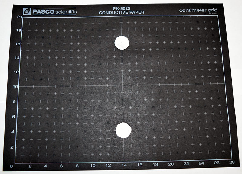
Initial setup.

1. Attach black paper to the cork board with aluminum pushpins through the conducting circles. Make sure the pushpins’ heads have good contact with the conducting circles on the paper.  


2. Attach alligator clip wires to the aluminum pushpins. Connect other ends of alligator clip wires to long jumper wires.  


3. Attach jumper wire connected to the “upper” circle to the “3.3V” terminal of your iOLab device. This disk will be at a (higher) potential of 3.3V.  


4. Attach jumper wire connected to the “lower” circle to the “GND” terminal of the iOLab device. This is the ground terminal, meaning it has a potential of 0 Volts. The suggested connection setup of “3.3V” and “GND” terminals is not essential for the experimental results but we will refer to this setup in our calculations.  


5. Attach additional jumper wire to the “A7” terminal and connect it to the third alligator clip wire. This wire will be your probe for the electric potential.  


6. Turn on your iOLab, activate the “Analog 7” probe and click “Record”. It should read about 1.65 V when it is not touching anything.  


7. You may click on the graph title “Analog 7”– this will collapse the graph and will conveniently show numerical value for the voltage measured by the probe.  

Measurements.

Part I.

1. First, we will explore how the electric potential varies as a function of position on the conducting paper. Measure the potential along the line connecting the circles at  intervals. Make appropriate table in Excel – potential vs. position (in cm). You may choose the origin at the midpoint between the circles (in this case the position would range from  to , with  having potential of  and  at about ).


2. Create a plot of your experimental data for potential vs. position.


3. Use Model 1 proposed for this experiment to calculate theoretical estimate for the potential vs. position and compare with your experimental results. Add additional column in your spreadsheet with calculated values of  for the same values of  as your experimental data (use  in your calculations).


4. Plot your calculated  on the same graph as your experimental results


5. Comment on your results. Do they match? If not, is the difference significant? What might be the reason for the discrepancy?


6. Estimate the magnitude of the electric field from your experimental data. For each point approximate the derivative of the potential with a finite difference:
      (you may calculate electric field magnitude in Volts/cm). Create additional column in your spreadsheet for your  estimate.


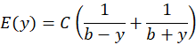
7. Create yet another column for theoretical values of  (use the value for coefficient  you found in Prelab for Model 1):
   


8. Plot your experimental and theoretical estimates of  on the same graph. Your experimental estimate may be noisy – it is ok.


9. Your report should contain graph with your experimental and calculated results for , the graph with your experimental and theoretical estimates of , and your reflections on the results and accuracy of the proposed Model 1.

Part II.

Plotting equipotential lines and electric field lines.

You will plot equipotential lines on the provided template that mimic your experimental setup (Figure E.2).

Drawing equipotential line:

Activate the “Analog 7” probe and click “Record”. Place alligator jumper wire connected to the A7 terminal at a point on the black paper.

Find a point on the black paper that has needed value of the potential. Mark corresponding point on the template. Glide the alligator wire along the paper to find a nearby point with the same potential, mark corresponding point on the template etc. Repeat until you have enough points to draw a smooth equipotential line through your points. Do not neglect points far from the circles and close to the edge of the sheet – make sure you draw an accurate equipotential curve all the way until the edge of the paper. It might take a little time to get a grip on it. Imagine how equipotential should look like and try to not move your probe at random but rather anticipate the shape of the equipotential. You may also use a symmetry – once you plotted the equipotential on one side of the axis of symmetry you may simply reflect the curve relative to the symmetry line.

1. Create equipotential diagram with the voltage steps of 0.15 Volts. Label equipotential lines with appropriate values of electric potential.


2. Draw the electric field lines on your equipotential diagram, indicating the direction of the electric field. Use different colors or line styles for the electric field lines and equipotentials.


3. From your equipotential data estimate the magnitude of the electric field at the middle point between the circles.


4. Your report should contain the scan/photo of your equipotentials and electric field diagram. Report your estimate of the electric field at the middle point between the circles. Does it match your estimates from part I?

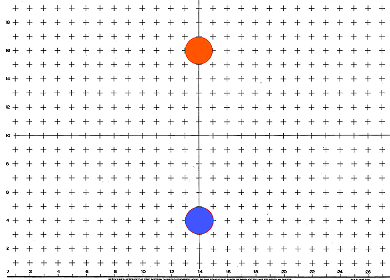
Experiment 2.

In this experiment you will work with the conducting paper that, in additional to the circles in Experiment 1, has a larger (radius 2cm) circle in the middle (Figure E.3).

1. Connect the lower circle to the Ground and the upper circle to the 3.3V terminal as in Experiment 1. Draw equipotential lines on the corresponding template (Figure E. 4) with the voltage steps of 0.15 Volts. Label equipotential lines with appropriate values of electric potential.


2. Draw the electric field lines on your equipotential diagram, indicating the direction of the electric field. Use different colors or line styles for the electric field lines and equipotentials.


3. Your report should contain the picture of your equipotentials and electric field diagram and your reflections on the behavior of equipotential lines and electric field lines in the vicinity of the conductor.

   

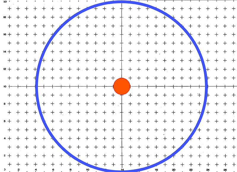
Experiment 3.

In this experiment you will work with the conducting paper that has a small (radius 1cm) circle at the center and large concentric circle of radius 10cm (Figure E.5). Connect small central circle to the 3.3V terminal of the iOLab. Connect the large circle to the ground terminal.

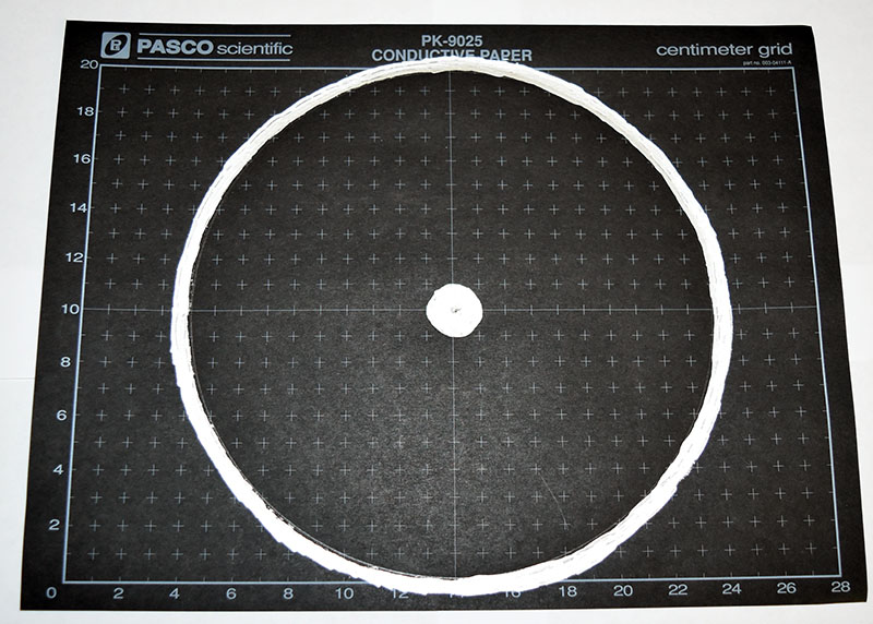
We have a circular symmetry in this setup. What shape do you anticipate for the equipotential lines? How should electric field lines look like?

1. Measure the electric potential along the radial line between concentric circles at 0.5cm intervals. Make appropriate table in Excel – potential vs. radial distance from the center of circles.


2. Draw equipotential lines on the corresponding template (Figure E.6) with the potential increment between the lines of 0.3V (use symmetry to draw your equipotential lines).





3. Draw the electric field lines on your equipotential diagram, indicating the direction of the electric field. Use different colors or line styles for the electric field lines and equipotentials.


4. Create a plot of your experimental data for potential vs. radial distance  from the center.


5. Calculate theoretical estimates for  using our Model 2. Plot calculated values for  on the same graph as your experimental results.


6. Comment on your results. Do they match? If not, is the difference significant? What might be the reason for the discrepancy?


7. Your report should contain the picture of your equipotentials and electric field diagram, the graph with your experimental and calculated results for , and your reflections on the results.