Model 1 Resistance between two disks on the infinite conducting plane.
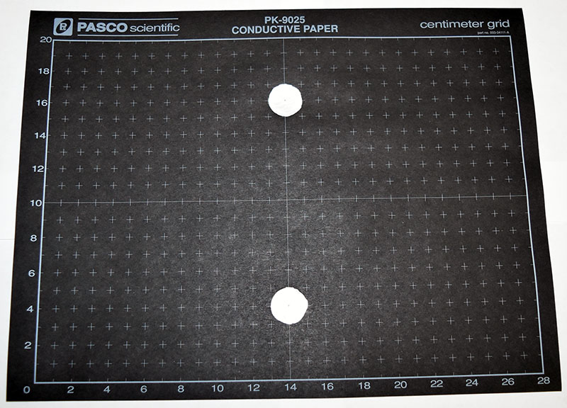
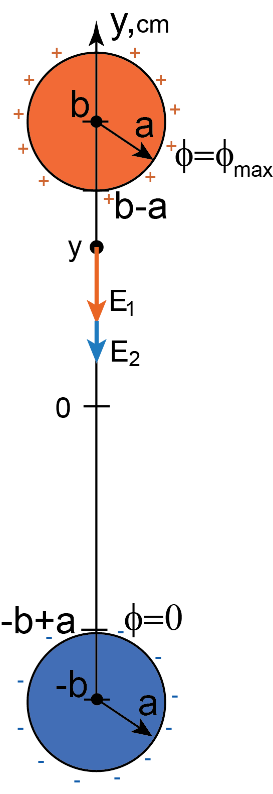
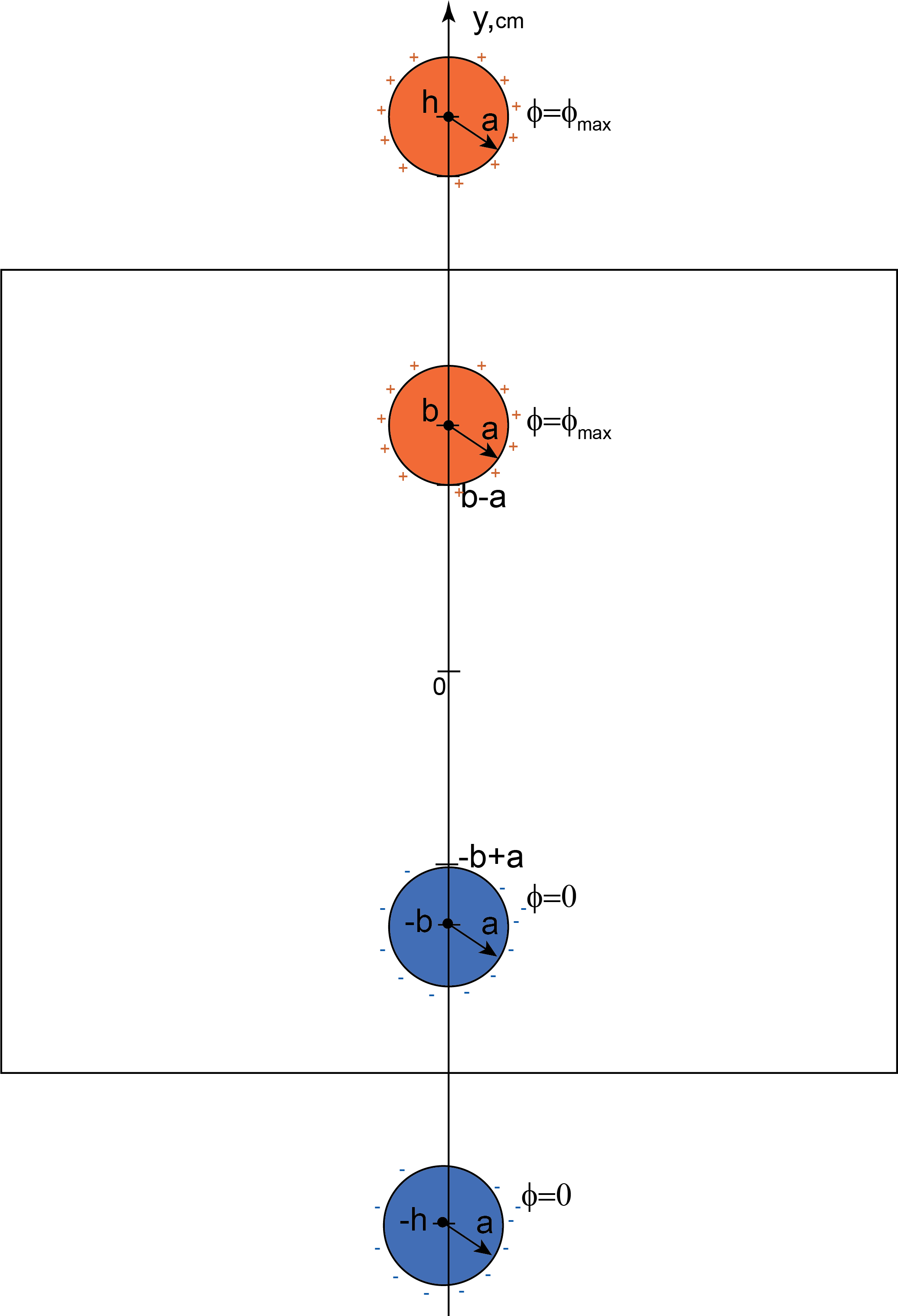
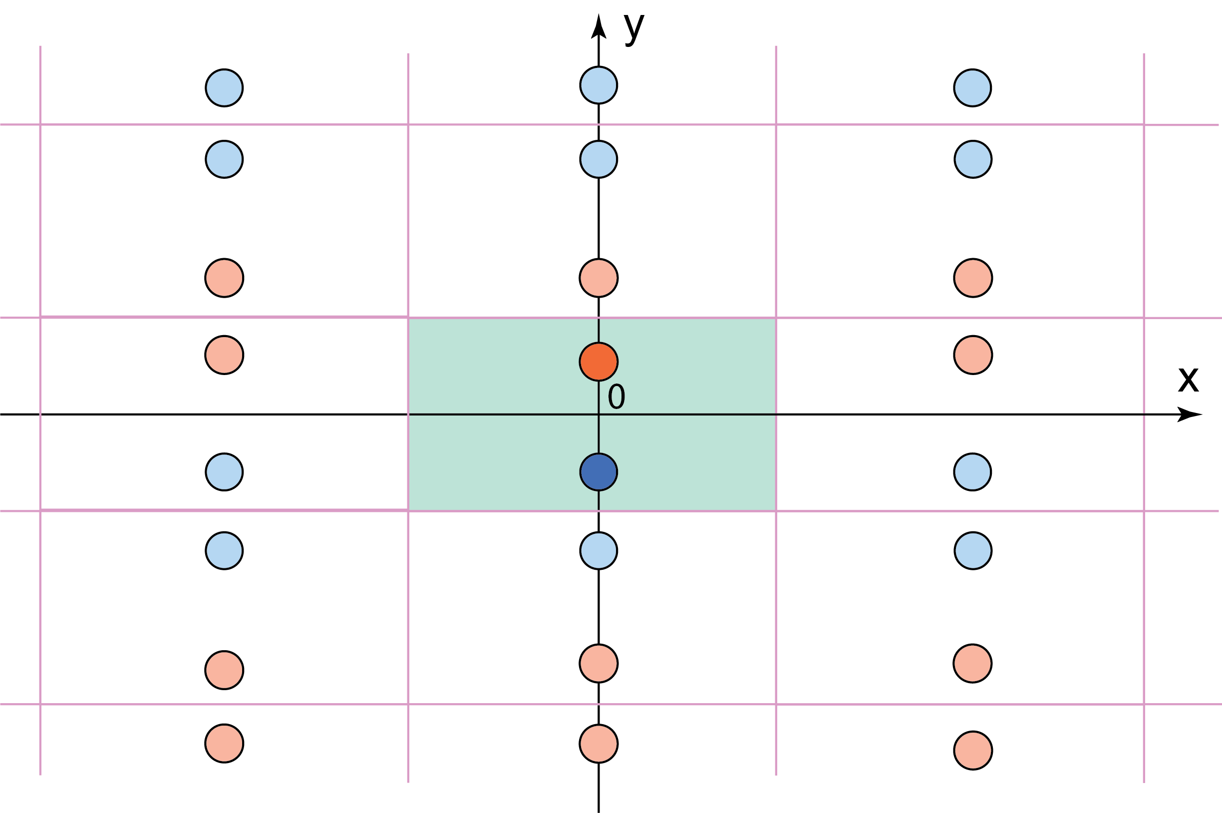
We consider electric field by two identical oppositely charged very thin disks on the plane (see Figure M.2). The charges on these circles are produced by connecting them to the voltage source that maintains known potential difference ![]() between them. This is a “2D” case – electric field lies in the plane of the disks. You may think of these disks as cross-sections of very long charged cylinders (due to translational symmetry electric field lies in the plane perpendicular to the axes of the cylinders).
between them. This is a “2D” case – electric field lies in the plane of the disks. You may think of these disks as cross-sections of very long charged cylinders (due to translational symmetry electric field lies in the plane perpendicular to the axes of the cylinders).
- Recall that in “2D” case the magnitude of the electric field due to charged disk is inversely proportional to the distance from its center:
- Let us determine the value of the constant
 . Assume the disks have radii
  and their centers lie on
  axis at points
  and
and  . Consider electric field at some point on the
  axis between the circles(see Figure M.2). We assume the “upper” circle is at potential
  while the “lower” circle is at 0 potential (connected to GND). Electric field at point
  due to “upper” positively charged disk is
 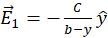 . Electric field at point
  due to “lower” negatively charged disk is
 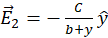 . Electric fields
  and
and  have the same direction therefore the net field at point
  is:
is:
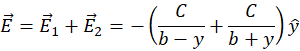
(M.2)
The difference in electric potential between the disks:

(M.3)
Integrate (M.3):

Express
 in terms of
  ,
,  ,
,  :
: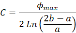
(M.4)
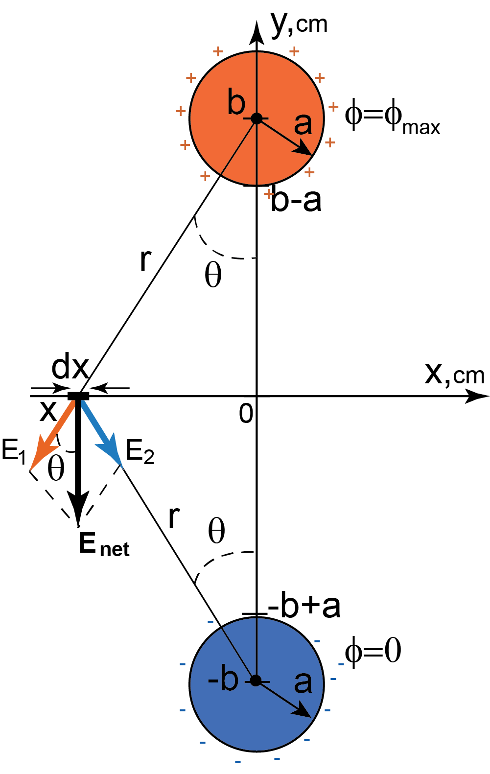
You derived this result in Prelab assignment for Lab 2. - Now consider a point on
 axis (see Figure M.3).
  axis is a symmetry line in our setup. Electric fields
  and
and  at this point due to “upper” and “lower” circles add up to the net field
  that has only
  component (due to symmetry). The magnitude of
  :
: - The current through the small segment
 is perpendicular to the
  axis and has the magnitude (see (I.6)):
 - Integrate (M.6) to obtain the net current crossing
 axis:
axis:
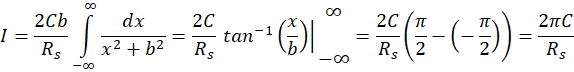
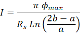
Plug in our expression for from (M.4):
 - Comparing (M.7) with Ohm’s Law
 we obtain expression for the resistance between two thin disks on the infinite conducting plane:
 - There is alternative (and shorter!) way to derive (M.8). Consider a circle of radius
 - i.e. a circle that contains one of our disks (positive, for example). The current flows radially outward through this circle. Therefore, the net current through the circle is (see (I.5))
  where
where  (i.e. the length of the line perpendicular to
  is just a circumference of the circle of radius
  since
since  is directed radially outward, i.e. perpendicular to the circle). Use (M.1) and (M.4) to express the magnitude of
  at distance
  from the center of the circle and obtain expression for the current in terms of
  ,
,  ,
,  ,
,  . Compare resulting expression for current with Ohm’s Law (as was done in part 6) and obtain expression for the resistance between two thin disks on the infinite conducting plane (M.8).
|
(M.1) |
|
(M.5) |
|
(M.6) |
|
(M.7) |
|
(M.8) |
What to submit in Prelab:
Your alternative derivation (from part 7) for the resistance between two thin disks on the infinite conducting plane (M.8).
Note
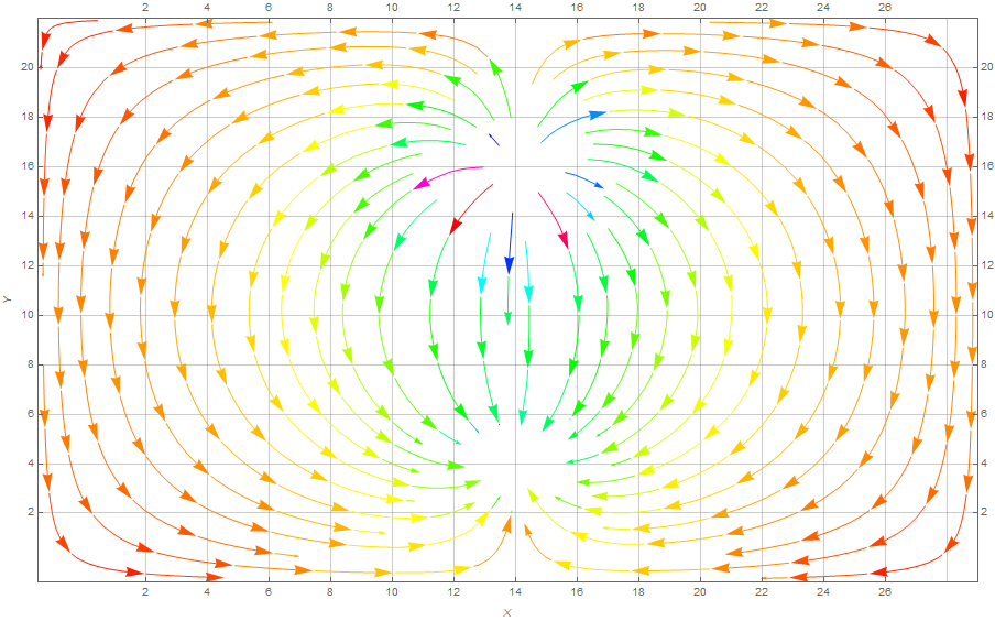
Electric field line crossing the boindary means, according to the Ohm’s law ![]() that some current leaves the sheet, which cannot happen.
that some current leaves the sheet, which cannot happen.
Another way to think about it – electric field lines crossing the boundary would violate the Gauss’s Law – if we draw a small closed surface around the boundary we end up with nonzero flux of electric field through that surface although there is no charge enclosed by such surface.
Current model does not consider the finiteness of the sheet and allows electric field lines to cross the boundary (see Figure M.5). This leads to some inaccuracy in its estimates for potential, electric field, current and resistance.
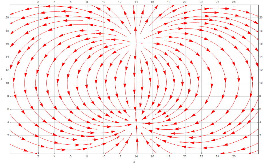
How can we adjust this Model to treat boundaries correctly? We may introduce images charges (see Figure M.6). Consider the upper boundary of the paper. Positive circle is located close to that boundary. We may place identical positive image circle above the boundary, so that both the positive circle and its image are symmetric with respect to the upper boundary. Electric field created by the positive circle and its image is parallel to the upper boundary everywhere at that boundary.
As we consider images located further away from our sheet their contributions to the electric field and the current decrease with their distance to the sheet. Therefore, as a good first approximation, we may consider only electric fields by the circles themselves and their nearest images (shown in Figure M.6). Calculations of the equivalent resistance of the finite sheet that take into account charged disks and their nearest images are very similar to our deviation in Model 1. You will not need to perform these calculations in this lab.
Model 2 Resistance between two concentric circles.
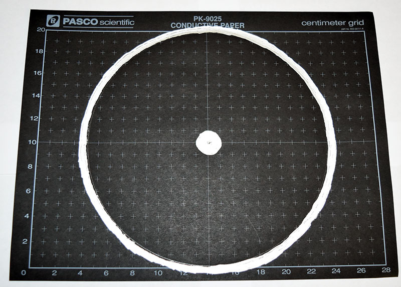
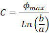
Assume the radius of the small circle is ![]() and the radius of the large circle is
and the radius of the large circle is ![]() . We will assume (as in Lab 2) that the small circle is at potential
. We will assume (as in Lab 2) that the small circle is at potential ![]() while the large circle is at potential 0 (see Figure M.9).
while the large circle is at potential 0 (see Figure M.9).
- Electric field in this setup is directed radially outward and, due to circular symmetry, is inversely proportional to the distance from the center:

(M.9)
- We need to find coefficient
 and express it in terms of
  ,
,  , and
, and . Express the difference in electric potential between the circles through the line integral of electric field along the radial line:
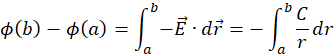
(M.10)
Integrate (M.10):
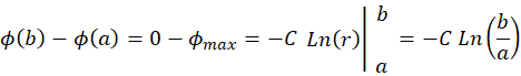
Express
 in terms of
  ,
,  ,
, :
:
(M.11)
You derived this result in Prelab assignment for Lab 2.
- Use (M.9) and (M.11) to express the magnitude of the electric field at distance
 from the center in terms of
  , a, b.
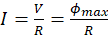
 - Now let us take a circle of arbitrary radius r:
 . The current flows radially outward through this circle. Therefore the net current
  through the circle may be calculated taking
  (i.e. the length of the line perpendicular to the
  is just a circumference of the circle of radius
  since
since  is directed outward, i.e. perpendicular to the circle). Obtain expression for the current in terms of
  ,
,  ,
,  ,
,  .
. - Compare your expression for the current with Ohm’s Law
 and obtain the expression for the resistance
 between the circles in terms of
  ,
,  ,
,  .
.
What to submit in Prelab:
- Your expression for the resistance
 between the circles with a short derivation.
 - Does this model suffer from the same failure to account for the finiteness of the sheet as Model 1? Do we need to introduce image charges in this model to ensure correct behavior of electric field at the boundaries?
Alternative derivation.
![]() and thickness
and thickness ![]() (Figure M.10). The current through the ring flows radially outward. Therefore, the resistance of this ring is
(Figure M.10). The current through the ring flows radially outward. Therefore, the resistance of this ring is
![]()
Here the ![]() is the "length" of the conductor (i.e. the extent of the conductor in the direction of the current),
is the "length" of the conductor (i.e. the extent of the conductor in the direction of the current), ![]() is the "width" of the conductor. It is the circumference of the ring:
is the "width" of the conductor. It is the circumference of the ring: ![]() (i.e. the extent of the conductor in the direction perpendicular to the current). Therefore:
(i.e. the extent of the conductor in the direction perpendicular to the current). Therefore:
![]()
We can subdivide the area in between our concentric circles on many such thin rings. These rings will all be "connected in series" as the current flows directly from one ring to the next. Therefore, the net resistance between our concentric circles of radii ![]() and
and ![]() is the sum, i.e. the integral of such
is the sum, i.e. the integral of such ![]() s. Integrate to obtain the net resistance. Compare with your expression for this resistance you obtained earlier.
s. Integrate to obtain the net resistance. Compare with your expression for this resistance you obtained earlier.
What to submit in Prelab:
- Your alternative derivation for the resistance between the concentric circles and your answers on the questions above.
- Not mandatory (extra credit). Can you always use the approach we used in the alternative derivation for this model – i.e. subdivide the object on many thin layers, find resistance of each thin layer and then add it up (integrate) to obtain the net resistance of the object? If not, under what circumstance can we use this approach? You might want to check homework problems 4.6 and 4.32 before you answer this.