Warnings! In this lab you will be provided with two neodymium magnets. Please read carefully the following warnings to understand precautions necessary whine handling these magnets.
Powerful attraction forces can cause injury.
Neodymium magnets are more powerful than other kinds of magnets. Very powerful attraction force between magnets can often be surprising to those unfamiliar with their strength. Fingers and other body parts can be pinched between two magnets.
Neodymium magnets can affect pacemakers.
The string magnetic fields near a neodymium magnet can affect pacemakers, ICDs and other implanted medical devices. Many of these devices are designed to deactivate in a magnetic field. Care must be taken to avoid inadvertently deactivating such devices.
Neodymium magnets can break.
Neodymium magnets are made of a hard, brittle metal. Despite the shiny. Metallic appearance of their nickel plating, they are not as durable as metal. Neodymium magnets can peel, chip, crack or shatter if allowed to slam together. Each magnet is marked by the arrow sign. Make sure you do not allow two magnets with the arrows pointing in the same directions to be close to each other. As a rule – either keep two magnets very far (at least 1 meter) apart, or carefully and controllably allow them to stick together. Do not let them slam into each other as the force of attraction is very large and shattering magnets can launch small pieces at great speeds.
Magnets can affect magnetic media.
The strong magnetic fields near neodymium magnets can damage magnetic media such as credit cards, magnetic ID cards and some electronic appliances.
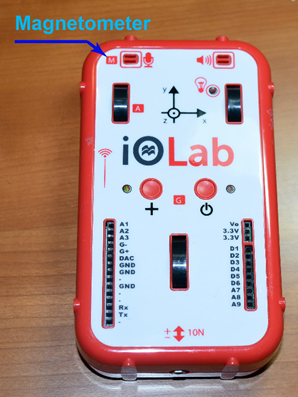
Figure E.1 Location of the Magnetometer on iOLab device.In this lab you will measure magnetic fields. These are delicate experiments so special care needs to be taken in order to avoid errors and interferences that may invalidate your results. Magnetometer sensor in the iOLab device is located under letter “M” in the upper left corner (see Figure 12).
Make sure all objects that may produce magnetic field are removed far away (at least a meter or more) from iOLab device. This includes computer monitors, batteries, and, especially, provided neodymium magnets. Check the absence of interfering magnetic field with the iOLab device (move it around in horizontal plane and observe that magnetic field does not noticeably change – i.e. there is no magnetic field beside terrestrial).
It may be hard to achieve the absence or interfering magnetic fields in Clough. I recommend doing Experiment 1 outside of the building.
Calibrate magnetometer often (before each experiment that involves measurement of the magnetic field). The calibration process is explained in the first experiment.
Device Calibration.
Before you start making measurements with iOLab ’s magnetic field sensor you need to calibrate this sensor. iOLab device relies on Earth’s magnetic field in the calibration of the magnetometer.
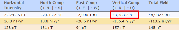
Go to https://www.ngdc.noaa.gov/geomag/calculators/magcalc.shtml#igrfwmm and enter the zip code of your location in the “Location” field. Click on the blue ”Get & Add Lat/Lon” button. You should see Latitude and Longitude fields on the left populated with your geographic location. Click on blue “Calculate” button in the bottom of the page. A new data panel will appear. You only need the value for the “Vertical Comp” – i.e. the vertical component of the Earth’s magnetic field at your location.
Figure E.2
Download the file config.json. Open it with text editor. Here is the content of this file:
{
"earthMagneticFieldZ": yourfield
}
Edit this file and replace “yourfield” with the numerical value for the vertical component of the Earth’s magnetic field at your location. Note: the value on the website in provided in while the value you need to put in config.json file is expected in . Convert in . Also note that the site gives the magnitude of the z-component of the magnetic field. Since we are in the Northern Hemisphere the z-component of the magnetic field is negative (i.e. directed downward) -see Figure I.6. Do not put any units in the file. Figure E.2 shows an example - magnetic field at my location. For this magnetic field, my config.json file is:
Figure E.3
{
"earthMagneticFieldZ": -43.38
}
Move config.json file in the “iOLab -WorkFiles” folder (which is in your Documents folder). Make sure your text editor does not add any extensions to this file. Note: you only need to make steps 1-3 of the calibration once – you will never need to touch config.json again.
Turn on iOLab device and start iOLab software. Click on Settings icon and then choose “Calibration” option (see Figure E.3). Select “Accel-magn-gyro” option. Follow the prompts.
Experiment 1: The Earth’s magnetic field.
Place your iOLab device flat on a table on wheels, engage magnetometer sensor and rotate the device slowly so that x-component of the magnetic field reads close to zero while y-component of the magnetic field is at its positive maximum.
Figure E.4
The y-axis (see the diagram on the device) of the iOLab is now pointing north.
Record magnitudes for both y- and z-components of the magnetic field (chose a time interval and use statistics tool to obtain the average of magnetic field components over that time interval).
Calculate the colatitude angle for your location (see Figure E.4). In your calculation assume that
The Earth's magnetic field is that of a magnetic dipole moment located at the center of the planet.
Ignore the difference between the geographic and magnetic poles - assume that the dipole moment is oriented North.
These assumptions allow us to use (I.9) to estimate colatitude and the magnitude of the Earth's magnetic dipole moment .
Calculate latitude for your location. Compare your exact latitude data from the website you used in calibration procedure with your calculated value. Comment on the accuracy of your calculation.
Calculate the magnitude of the Earth's magnetic dipole moment .
Your report should contain your calculations for the latitude, magnitude of , and your comments on the comparison of your calculated latitude value with the exact data.
Experiment 2: Measurement of magnetic dipole moments of permanent magnets.
In this experiment we will measure magnetic dipole moments of two neodymium magnets. Please read warnings and use precautions while working with these magnets as they are quite strong! You have two magnets in your lab kits – one has blue color on its top surface, and another is black. Magnets have the same mass and dimensions but slightly different magnetic dipole moments.
Place iOLab device on its wheels. Turn it around and identify the position such that (east-west). Your device will move along its y-axis and measure magnetic field and distance traveled. Make sure that the area you conduct this experiment is (mostly) free of not-terrestrial magnetic fields - move if along y-axis a little and check that stays close to zero
Place a blue magnet at a large distance (>1m) from the iOLab such that it is on the y-axis of the device (i.e. iOLab will approach the magnet such that magnetic sensor is moving right toward the magnet). You may elevate the magnet a little so that its axis is aligned with the y-axis of iOLab magnetometer sensor.
In the iOLab menu select “Magnetometer” and “Wheel”. Select and “Position”. Start moving iOLab device slowly toward the magnet. Observe By increasing. You may stop when goes off the chart. You do not need to go all the way to the magnet, in fact it is not recommended. Note approximate distance between the iOLab and the magnet at the moment when you stop your measurement.
Log into cloud storage and upload your experimental data there (click on button in the menu). Find your data in the cloud storage and download it from the cloud in CSV format. We do not use “Export to CSV” option in the iOLab software because different sensors in the device work at different frequencies. For example, magnetometer works on frequency 80Hz (i.e. it records 80 measurements for the magnetic field each second). The position sensor works on frequency 100Hz. It is tedious to build a simple magnetic field vs. position function with such data. Uploading to the cloud automatically synchronizes all sensor data.
Open your CSV file in Excel. Remove unnecessary data and make the and position data positive. Make a plot of the magnetic field vs. distance traveled by the iOLab device.
Now we will compare our experimental data with in (I.9) and calculate the magnetic dipole moment magnitude of our magnet. Since we measure magnetic field on the axis of the dipole .
Figure E.5
Let us call the total distance traveled by the iOLab device towards the magnet . This distance is just the last value in the position column. Assume that after traveling distance the iOLab device stopped at distance from the magnet (the distance of closest approach, see Figure E.5). Therefore, when the iOLab device traveled distance towards the magnet it is at the distance from the magnet. Create a cell in your spreadsheet for and populate it with some initial value. Do not worry about not knowing it exactly. Create another cell in your spreadsheet for magnetic dipole moment and populate it with another initial value.
Using (I.9), and known values create a column for theoretical values of . Fit your experimental data to your theoretical expression in Excel using Solver. Use both and as your fitting parameters.
Plot your optimized theoretical on the same graph as your experimental data. What are your and ? Does your value for match the distance between the iOLab and the magnet at the moment when you stopped your measurement (the point of closest approach)?
Repeat the measurement and calculation of for the second (black) magnet.
Your report should contain your results for magnetic dipole moments, comparison of you optimized with your experimental observations, and graphs with experimental and theoretical for each magnet.
Experiment 3: Magnetic levitation
In this experiment we will again measure magnetic dipole moments of our magnets.
Figure E.6 Measurement of the ratio of the magnetic dipole moments.
At first, we will measure the ratio of the magnetic dipole moments: . Place iOLab device on the table and rotate it into the position where . Place a short plastic tube from your kit on the table next to the iOLab device. Align the tube along the y-axis of the device and secure it on the table with the scotch tape. Place the blue magnet in the tube at the end opposite to the device such that the magnet is even with the end of the tube (see Figure E.6). Record the value for (select certain time interval and record the mean over that interval). Remove blue magnet from the tube and repeat this procedure with the black magnet. Calculate the ratio of values registered for black and blue magnets:. Include this ratio in your report. The plastic tube was used to secure both magnets in exactly the same position. Was it important to conduct this experiment in the area free of other magnetic fields (like computers or other sources beside the Earth’s magnetic field)?
Figure E.7
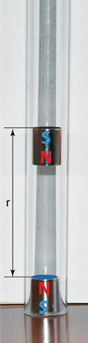
Place one magnet in the short plastic tube and position the tube vertically on the table. Orient the second magnet oppositely to the first one (so that the magnets would repel each other) and also place it in the tube. The second magnet will levitate in the magnetic field created by the first magnet, the repulsive magnetic force on the levitating magnet cancels with the force of gravity (see Figure E.7).
Use suppled ruler to measure the distance between the magnets.
Use (I.12) and from (I.9) with to derive expression for the magnitude of the repulsive (or attractive – depending on their orientation) force between two magnetic dipoles at distance from each other. Express the force magnitude in terms of and (since , and you know the ratio of the magnetic dipole moments from step 1)
Draw free body diagram for the levitating magnet and derive the expression for the magnetic dipole moment of the blue magnet.
The masses of the magnets are identical: 9.24 g. Calculate and . Compare with your results from Experiment 2.
Your report should have your derivation for and comparison of magnetic dipole moments values obtained in this Experiment with the results of Experiment 2. Does the distance between magnets in this experiment depend on which magnet levitates and which is at the bottom of the tube? Explain (magnets have identical masses but different magnetic moments).
Experiment 4: The force between magnetic dipoles.
The experimental setup is similar to the previous experiment. Place two oppositely oriented magnets (magnetic dipoles) in the short plastic tube – this time placed horizontally on the table. You will then measure the repulsive force between the magnets as a function of distance between them and calculate their magnetic moments.
Screw the eye-bolt or the small disk into the force probe of the iOLab device. Calibrate the force sensor on the device. Calibration of the force sensor is similar to the calibration of the Magnetometer – just select the Force option in the Calibration menu and follow the prompts.
Place one magnet in the tube and position the tube horizontally on the table against something heavy (and nonmagnetic) so that one end of the tube is blocked. Orient the second magnet oppositely to the first one (so that they would repel each other) and also place it in the tube.
Figure E.8
Insert short wooden rod in the tube so that the rod is in between the second magnet and the force sensor of the iOLab device (see Figure E.8).
In the iOLab software menu select “Force” and “Wheel”. In the “Wheel” submenu select position only.
Push slowly on the iOLab device and observe the force increase. You may push until the force is off the chart (i.e. the force magnitude is about 5N). Make a note of the “distance of the closest approach” – i.e. the minimal distance between the magnets when you stopped pushing.
Upload your experimental data to the cloud and download it from there in CSV format. Open in Excel and remove unnecessary data preceding the start of the measurement (when iOLab was not moving) and after the measurement (when iOLab moves back and the Force is decreasing). Make the position data positive.
Now we will compare the experimental data with the theoretical expression for the force. We will use the same approach as in Experiment 2. Let us assume the total distance traveled by the iOLab device (i.e. the last value in the position column) is . At the moment when iOLab traveled distance the distance between the magnets is where is again the distance between the magnets at their closest approach. Create cells in your spreadsheet for and and populate them with initial values.
Using the expression you derived in the Experiment 3 for the force between magnetic dipoles and at distance from each other create a column for theoretical values of the Force. Use value known from Experiment 3. Fit your experimental data for the Force between two magnets to your theoretical expression using Solver. Use and as your fitting parameters.
Your report. Plot your optimized theoretical ) on the same graph as your experimental data for the Force and include in your report. What are and ? Does your value for match the observed distance of the closest approach between two magnets? Compare and obtained in this experiment with corresponding values from Experiments 2 and 3.
Experiment 5: Electric Motor.
Figure E.9 The basic setup of a simple electric motor.
In this Experiment you will build primitive electric motor and study its frequency characteristics.
The magnetic force on the current-carrying wire (I.2) is the main principle behind operation of our simple motor. The basic setup is shown in Figure (E.9). A coil of n=3 (strictly speaking 3.5) turns of isolated wire is suspended between two conducting axle supports made of stripped wire and secured on the breadboard. The coil can rotate freely about its axis. The magnet is placed on the breadboard under the coil such that as the coil rotates it gets close to the magnet without touching it.
Assume there is a current in the coil. For simplicity imagine the coil at the moment when it is in the vertical plane. The lower side of the coil that is closer to the magnet experiences a force directed perpendicular to the plane of the coil. The upper side of the coil experiences a force in the opposite direction and the magnitude of this force is smaller than that of the force on the lower side due to weaker magnetic field. We see that the coil experiences a torque that rotates the coil about its axis. The magnitude of the torque is proportional to both the magnitude of the magnetic field and the current in the coil (see (I.2)).
Can we expect a coil with constant current to rotate through one revolution due to magnetic torque? No.
Consider a situation after the coil makes a half rotation about the axle. The coil is again in the vertical plane but the sides swapped places - the side that was closer to the magnet is now farther from it while the side that was farther from the magnet is now closer to it. Since current runs in opposite directions in two sides of the coil after half rotation the torque on the coil reverses direction. This should, in principle, reverse the rotation of the coil, so that it would oscillate rather than spin about its axle. For an electric motor to work, the current in the coil should reverse direction every half turn, which requires more sophisticated contacts between the axle and the support. Or, if the current were shut off every half turn of the coil, the motor could also work. Therefore, we need to shut off current approximately every ½ turn. We can achieve this by interrupting the contact between the conducting axle supports and the coil every ½ turn. For this reason, we strip one end of the coil wire only partially, from one side only (see Figure E.9). As the coil rotates the remaining isolation periodically interrupts the contact and the current stops. Maximum efficiency is achieved if the current in the circuit runs when one of the sides of the coil is in its lowest position (i.e. closer to the magnet). You may tweak and adjust the coil and the timing of current interruption to achieve fast-running motor.
Figure E.10 Motor Coil.
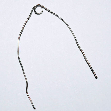
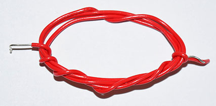
In your kit you have 18” piece of red wire that is stripped on one end and half-stripped on another end. Use this wire to make a coil with 3.5 full turns such that the ends of the wire stick out on opposite sides (see Figure E.10).
Extract a core from some pen and wrap provided short piece of the stripped wire around pen core once to make a single turn in the middle of the wire. This is your axle support. (see Figure E.11). Make the second axle support the same way.
Install axle supports on the breadboard. Install your coil on axle supports. Make sure the coil is well balanced and can rotate freely. Adjust and tweak your coil if necessary.
Figure E.11 Axle support
Place black magnet on the breadboard underneath your coil. Make sure your coil can rotate freely without touching the magnet. The coil should come close to the magnet without making contact with it. Tweak flexible axle supports if necessary.
Remove the magnet and assemble the circuit shown in Figure E.12 on the breadboard. Use AA battery as a voltage source. Connect A1 and ground terminals of the iOLab device across one of the resistors. Make sure that A1 terminal is connected at the point with higher potential than the point where you connect the ground (one example of such connection is shown in Figure E.12).
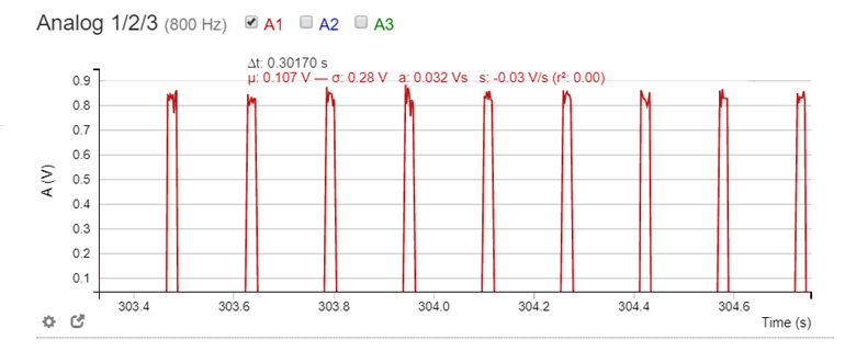
Activate “Analog 1/2/3” sensor in the iOLab software. Push your coil a little. You should observe peaks in the voltage across resistor as the current turns on and off by the half-stripped coil wire end. If you do not observe such periodic peaks check your circuit.
Place black magnet underneath the coil and push the coil. Hopefully, it starts rotating. If the coil does not rotate or rotates very slowly and then stops, try these tweaks:
Figure E.12 Motor circuit
Push the coil in opposite direction.
Move the magnet on the breadboard to find optimal position where coil rotates faster.
Turn magnet upside down (i.e. swap magnet poles). I recommend doing this even if your coil rotates – the coil rotates faster with one pole configuration.
Tweak (rotate) the half-stripped end of the coil to adjust the timing of its contact with the axle support.
Strip a little more isolation on the half-stripped end.
As the coil rotates you should observe periodic current in the coil registered as voltage peaks across resistor. Collect the data and enjoy your motor running for about ½ minute (Tip: avoid running this motor for long time as it will drain the battery. Think about magnitude of the current in your circuit).
With your motor running short-circuit one resistor (the one across which you do not measure the voltage) with a short jumper wire. The current in the circuit should increase and the coil should rotate faster. Collect data for another ½ minute.
Did the current in the circuit doubled when you short-circuited one of two resistors? Explain why. Tip: resistance of jumper wire, axle supports, and the coil itself is negligible compared with resistance.
From the measured data find (approximately) the maximum currents and in the circuits with two and one resistors.
Figure E.13
Now we will determine the frequency of the motor (with two and one resistors in the circuit). There are two ways to determine frequency from the data:
You may zoom in onto particular time interval and count the number of voltage peaks during known time interval (see Figure E.13). The frequency we are looking for is the number of peaks (i.e. number of coil revolutions) per one second. It is measured in .
There is a faster and more elegant approach –Fourier transform (FT) of the data.
Figure E.15Figure E.14
This is a mathematical transform that decomposes a signal or a function (of time) into its constituent frequencies. Original function is represented as a sum of many harmonic functions - sines and cosines with various frequencies. Fourier transform provides amplitudes for such harmonic functions. Since our signal is to a large degree periodic, we expect to see peaks in the amplitudes of the harmonic functions for the frequencies that are multiples of the fundamental frequency – the revolution frequency we are looking for. When original function (signal) is discrete it is best to apply Fast Fourier Transform (FFT) algorithm.
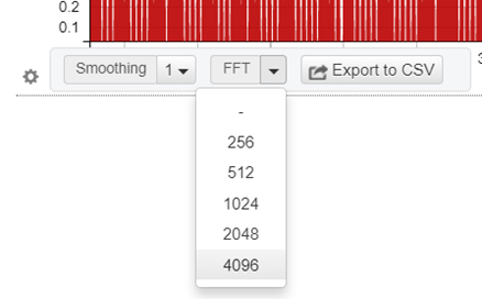
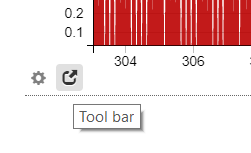
The iOLab software makes it very easy to apply FFT on the signal data. Click on the Tool Bar icon under your data graph (see Figure E.14). In the menu that will appear click on “FFT” submenu and select “4096” (see Figure E.15). This number represents the number of data points that will be analyzed.
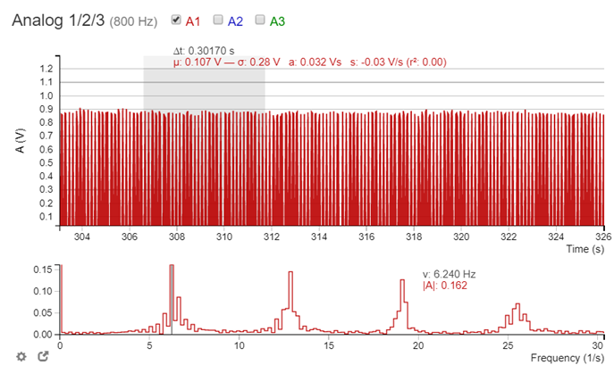
Figure E.16 The original signal and its FFT transform
You will see additional graph under your signal – this is a part of your data (4096 data points, to be exact) in the “frequency domain” – i.e. amplitudes of the harmonic functions vs. their frequencies. The region of the original signal that is transformed into frequency domain is highlighted in grey (see Figure E.16). You may click on that highlighted region and move it to change the time interval for the data shown in the frequency domain – play with it a little, it is fun and instructive. Choose such a region in the original data that produces the most clear peaks in the frequency domain (like in Figure E.16). The smallest frequency at which FFT transform exhibits a peak is our fundamental frequency – i.e. the coil revolution frequency. In the example shown in Figure E.16 this frequency is 6.240Hz.
Measure the motor coil frequencies and for two and one resistors in the circuit.
Compare the ratios and . Are they close?
Here is a simple theoretical model for the dependency of the coil frequency of our electric motor in this experiment on the current .
The work done on the coil as it accelerates (its rotation) in the magnetic field is proportional to the torque of the magnetic force which, in turn, is proportional to both the current and magnetic field magnitude as follows from (I.2). Therefore, the energy delivered to the coil in a single rotation is . Here is some coefficient of appropriate dimension. This energy is dissipated into heat through the work of retarding forces during the same rotation. There are two retarding forces at play here – the friction in the axle supports and the air resistance. Since the coil is very light the first one is (much) smaller than the second. Therefore, we will disregard the constant friction force in the axle supports and only consider air resistance. The magnitude of the air resistance force acting on the object moving with (a relatively low) speed is proportional to that speed: where is the constant of appropriate dimension that depends on the shape of the object. For the rotating coil, the retarding torque of the air resistance is therefore where is another constant and is angular velocity of rotation. I disregard the variability in the angular velocity of the coil during one revolution and assume it rotates with constant (average) angular speed . Since the retarding torque is . The magnitude of the work done by this retarding torque on the coil (i.e. amount of energy dissipated into heat) in one revolution (i.e. over the angular displacement ) is . Equating the energy delivered to the coil in one rotation to the energy dissipated on heat during the same rotation yields:
Therefore: .
Do the ratios you calculated in part 14 agree with the conclusion of this simple model?
Include in your report:
The screenshot of your signal (voltage across resistor) used for frequency calculation - in either Figure E.13 or Figure E.16 format (or both).
Your results for motor coil frequencies and and peak currents and .
Comparison of ratios and and your opinion on the validity of the model described in part 15.
Do not disassemble the coil and axle supports. You will need them for the next lab.
 while the value you need to put in config.json file is expected in
  . Convert
  in
in  . Also note that the site gives the magnitude of the z-component of the magnetic field. Since we are in the Northern Hemisphere the z-component of the magnetic field is negative (i.e. directed downward) -see Figure I.6. Do not put any units in the file. Figure E.2 shows an example - magnetic field at my location. For this magnetic field, my config.json file is:
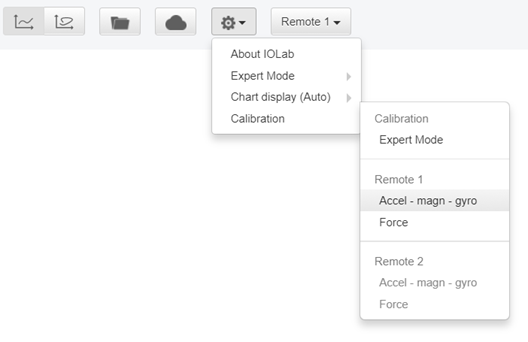
 for your location (see Figure E.4). In your calculation assume that
 located at the center of the planet.
 is oriented North.
 .
.
 .
. , and your comments on the comparison of your calculated latitude value with the exact data.
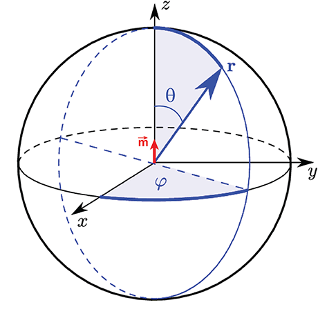
 (east-west). Your device will move along its y-axis and measure magnetic field and distance traveled. Make sure that the area you conduct this experiment is (mostly) free of not-terrestrial magnetic fields - move if along y-axis a little and check that
  stays close to zero
 and “Position”. Start moving iOLab device slowly toward the magnet. Observe By increasing. You may stop when
  goes off the chart. You do not need to go all the way to the magnet, in fact it is not recommended. Note approximate distance between the iOLab and the magnet at the moment when you stop your measurement.
  button in the menu). Find your data in the cloud storage and download it from the cloud in CSV format. We do not use “Export to CSV” option in the iOLab software because different sensors in the device work at different frequencies. For example, magnetometer works on frequency 80Hz (i.e. it records 80 measurements for the magnetic field each second). The position sensor works on frequency 100Hz. It is tedious to build a simple magnetic field vs. position function with such data. Uploading to the cloud automatically synchronizes all sensor data.
  and position data positive. Make a plot of the magnetic field
  vs. distance
  traveled by the iOLab device.
 in (I.9) and calculate the magnetic dipole moment magnitude
  of our magnet. Since we measure magnetic field on the axis of the dipole
  .
.  . This distance is just the last
  value in the position column. Assume that after traveling distance
  the iOLab device stopped at distance
  from the magnet (the distance of closest approach, see Figure E.5). Therefore, when the iOLab device traveled distance
  towards the magnet it is at the distance
  from the magnet. Create a cell in your spreadsheet for
  and populate it with some initial value. Do not worry about not knowing it exactly. Create another cell in your spreadsheet for magnetic dipole moment
  and populate it with another initial value.
 and known
  values create a column for theoretical values of
  . Fit your experimental data
  to your theoretical expression in Excel using Solver. Use both
  and
and  as your fitting parameters.
  on the same graph as your experimental data. What are your
  and
and  ? Does your value for
  match the distance between the iOLab and the magnet at the moment when you stopped your measurement (the point of closest approach)?
 for the second (black) magnet.
 with your experimental observations, and graphs with experimental and theoretical
  for each magnet.
 . Place iOLab device on the table and rotate it into the position where
  . Place a short plastic tube from your kit on the table next to the iOLab device. Align the tube along the y-axis of the device and secure it on the table with the scotch tape. Place the blue magnet in the tube at the end opposite to the device such that the magnet is even with the end of the tube (see Figure E.6). Record the value for
  (select certain time interval and record the mean over that interval). Remove blue magnet from the tube and repeat this procedure with the black magnet. Calculate the ratio of
  values registered for black and blue magnets:
 . Include this ratio in your report. The plastic tube was used to secure both magnets in exactly the same position. Was it important to conduct this experiment in the area free of other magnetic fields (like computers or other sources beside the Earth’s magnetic field)?
 between the magnets.
 from (I.9) with
  to derive expression for the magnitude of the repulsive (or attractive – depending on their orientation) force between two magnetic dipoles at distance
  from each other. Express the force magnitude in terms of
  and
and  (since
 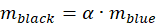 , and you know the ratio of the magnetic dipole moments
  from step 1)
 of the blue magnet.
  and
and  . Compare with your results from Experiment 2.
  and comparison of magnetic dipole moments values obtained in this Experiment with the results of Experiment 2. Does the distance between magnets in this experiment depend on which magnet levitates and which is at the bottom of the tube? Explain (magnets have identical masses but different magnetic moments).
 value in the position column) is
  . At the moment when iOLab traveled distance
  the distance between the magnets is
 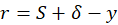 where
where  is again the distance between the magnets at their closest approach. Create cells in your spreadsheet for
  and
and  and populate them with initial values.
  and
and  at distance
  from each other create a column for theoretical values of the Force. Use
  value known from Experiment 3. Fit your experimental data for the Force between two magnets to your theoretical expression using Solver. Use
  and
and  as your fitting parameters.
  ) on the same graph as your experimental data for the Force and include in your report. What are
  and
and  ? Does your value for
  match the observed distance of the closest approach between two magnets? Compare
  and
and  obtained in this experiment with corresponding values from Experiments 2 and 3.
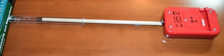
 resistors. Make sure that A1 terminal is connected at the point with higher potential than the point where you connect the ground (one example of such connection is shown in Figure E.12).
 resistor as the current turns on and off by the half-stripped coil wire end. If you do not observe such periodic peaks check your circuit.
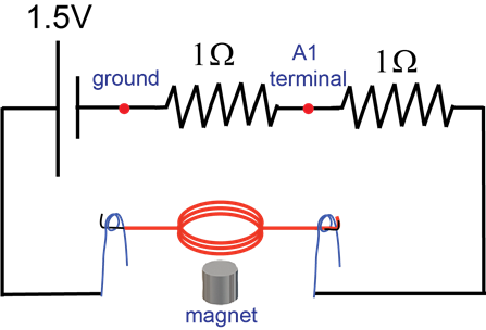
 resistor. Collect the data and enjoy your motor running for about ½ minute (Tip: avoid running this motor for long time as it will drain the battery. Think about magnitude of the current in your circuit).
 resistor (the one across which you do not measure the voltage) with a short jumper wire. The current in the circuit should increase and the coil should rotate faster. Collect data for another ½ minute.
  resistors? Explain why. Tip: resistance of jumper wire, axle supports, and the coil itself is negligible compared with
  resistance.
  and
and  in the circuits with two and one
  resistors.
  resistors in the circuit). There are two ways to determine frequency from the data:
 .
. 
 and
and  for two and one
  resistors in the circuit.
  and
and  . Are they close?
 of our electric motor in this experiment on the current
  .
. . Here
  is some coefficient of appropriate dimension. This energy is dissipated into heat through the work of retarding forces during the same rotation. There are two retarding forces at play here – the friction in the axle supports and the air resistance. Since the coil is very light the first one is (much) smaller than the second. Therefore, we will disregard the constant friction force in the axle supports and only consider air resistance. The magnitude of the air resistance force acting on the object moving with (a relatively low) speed
  is proportional to that speed:
  where
where  is the constant of appropriate dimension that depends on the shape of the object. For the rotating coil, the retarding torque of the air resistance is therefore
  where
where  is another constant and
  is angular velocity of rotation. I disregard the variability in the angular velocity of the coil during one revolution and assume it rotates with constant (average) angular speed
  . Since
  the retarding torque is
  . The magnitude of the work done by this retarding torque on the coil (i.e. amount of energy dissipated into heat) in one revolution (i.e. over the angular displacement
  ) is
) is  . Equating the energy delivered to the coil in one rotation to the energy dissipated on heat during the same rotation yields:
 .
. resistor) used for frequency calculation - in either Figure E.13 or Figure E.16 format (or both).
 and
and  and peak currents
  and
and  .
. and
and  and your opinion on the validity of the model described in part 15.