Model 1.
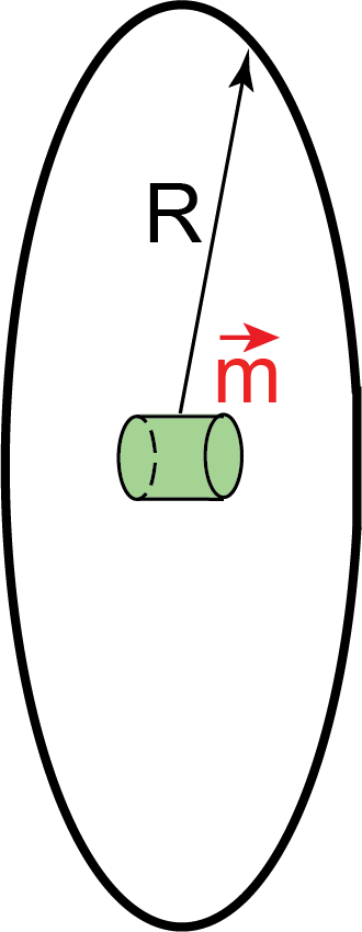
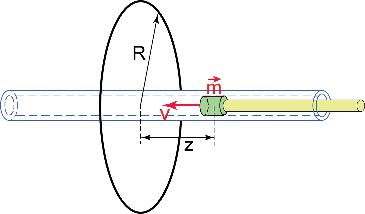
Assume a small magnet moves along a line perpendicular to the plane of the loop of radius
-
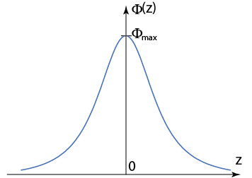
Magnetic flux through the loop is the same when the magnet is at the points that are symmetric with respect to the plane of the loop:
 . Therefore
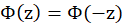
  is an even function.
 -
Magnetic flux through the loop is maximum when the magnet crosses the plane of the loop:
 .
. - Magnetic flux vanishes at large distance from the loop:
 as
as  .
.
Figure M.3 depicts a function that has these properties.
The flux of the magnetic field of the dipole moving along the axis of symmetry of the loop is given by (I.11) which we obtained by integrating the vector potential over the loop:
|
(M.1) |
It is easy to see that (M.1) satisfies all aforementioned properties and is of the shape shown in Figure M.3.
Our goal is to find the maximum value of the flux ![]() when the magnet passes through the center of the loop. As the magnet moves along the line perpendicular to the plane of the loop the induced emf in the loop as a function of time is (we do not watch for the signs here):
when the magnet passes through the center of the loop. As the magnet moves along the line perpendicular to the plane of the loop the induced emf in the loop as a function of time is (we do not watch for the signs here):
|
(M.2) |
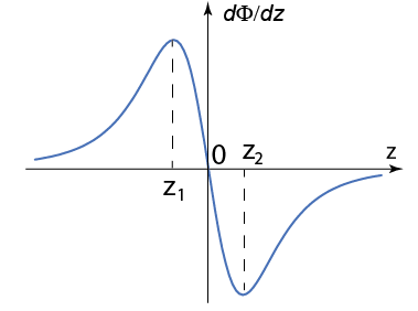
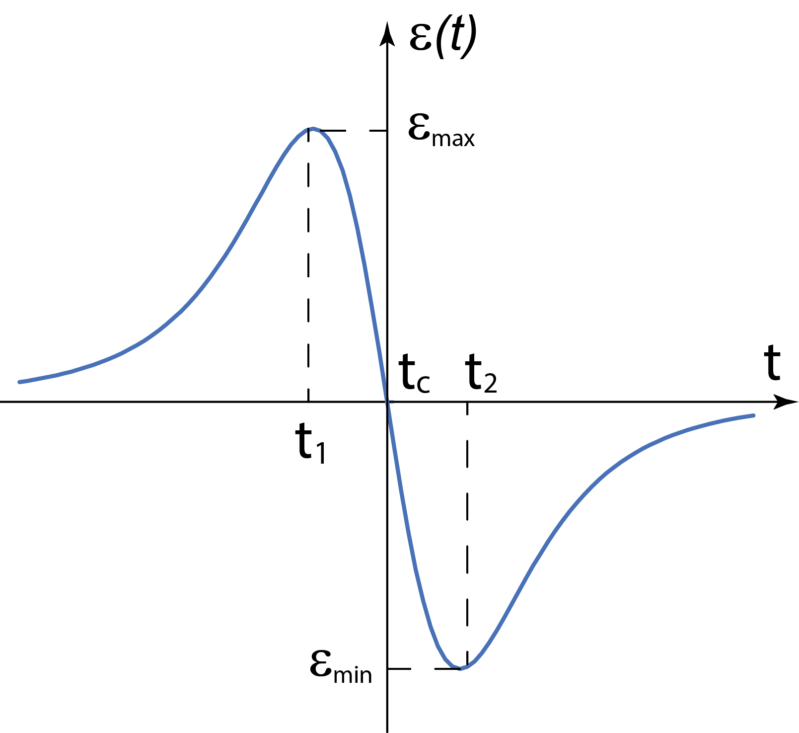
where ![]() is the speed of the magnet. The derivative of the function of the shape of Figure M.3 is shown in Figure M.4.
is the speed of the magnet. The derivative of the function of the shape of Figure M.3 is shown in Figure M.4.
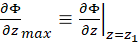
![]() has maximum at
has maximum at ![]() its derivative
its derivative ![]() at
at ![]() .If the sped of the magnet stays approximately constant as it moves through the vicinity of the loop
.If the sped of the magnet stays approximately constant as it moves through the vicinity of the loop ![]() the shape of the
the shape of the ![]() function mimics that of
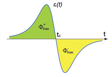
function mimics that of ![]() as follows from Faraday’s Law (M.2) (see figure M.5). Let us denote the time when the magnet crosses the plane of the loop
as follows from Faraday’s Law (M.2) (see figure M.5). Let us denote the time when the magnet crosses the plane of the loop ![]() . From (M.2) it follows that
. From (M.2) it follows that ![]() Integrating emf (M.2) with respect to time from
Integrating emf (M.2) with respect to time from ![]() to
to ![]() yields
yields ![]() :
:
|
(M.3) |
Therefore the flux through the circular loop of the magnetic field of the small magnet in the center of the loop is the integral of the induced emf in the loop with respect to time as the magnet moves from a very distant point to the center of the loop along the loop’s axis – this is the area under the ![]() curve from negative infinity up to the time
curve from negative infinity up to the time ![]() where
where ![]() crosses zero (
crosses zero (![]() shown in green in Figure M.5). We may also integrate
shown in green in Figure M.5). We may also integrate ![]() from
from ![]() to
to ![]() :
:
|
(M.4) |
The values for ![]() obtained from (M.3) and (M.4) should, in theory, be the same. Unfortunately, iOLab device has small bias for such measurements on High Gain terminal. This means that the
obtained from (M.3) and (M.4) should, in theory, be the same. Unfortunately, iOLab device has small bias for such measurements on High Gain terminal. This means that the ![]() curve is shifted a little – ether up or down. Because of this shift the values for
curve is shifted a little – ether up or down. Because of this shift the values for ![]() obtained through integration (M.3) from
obtained through integration (M.3) from ![]() to
to ![]() (
(![]() in Figure M.5) and through integration (M.4) from
in Figure M.5) and through integration (M.4) from ![]() to
to ![]() (
(![]() in Figure M.5) are slightly different. To exclude this bias, we will take the average of these flux values:
in Figure M.5) are slightly different. To exclude this bias, we will take the average of these flux values:
|
(M.5) |
For the magnet moving along loop’s axis of symmetry equating ![]() obtained through (M.5) with the value for
obtained through (M.5) with the value for ![]() from (M.1) allows to evaluate the magnetic dipole moment
from (M.1) allows to evaluate the magnetic dipole moment ![]() . You may compare it with the values you obtained using other techniques in Lab 5. I believe that the value for
. You may compare it with the values you obtained using other techniques in Lab 5. I believe that the value for ![]() obtained in this Experiment is more accurate (closer to the true value) than the values you calculated in Lab 5.
obtained in this Experiment is more accurate (closer to the true value) than the values you calculated in Lab 5.
Model 2.
Our goal is to express the magnetic dipole moment ![]() in terms of emf amplitude
in terms of emf amplitude ![]() .
.
-
At first, we need to find
 values where
  is maximum (
 and
and  in Figure M.4). From symmetry it is clear that
  .
.
-
Differentiate (M.1) with respect to
 to find the expression for
  .
. -
Differentiate
 with respect to
  to find
  .
. -
Solve equation
 to find
  and
and  where
where  attains its maximum/minimum values. Express
  and
and  in terms of loop radius
  .
.
-
Differentiate (M.1) with respect to
- Calculate
 . It is clear that
 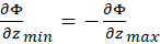 .
. -
From Faraday’s Law (M.2), it follows that
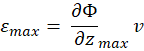
(M.6)
We will assume the magnet moves with constant speed over the interval
 (note: the time interval
  is very small). Therefore, we may approximate the speed of the magnet as
 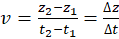 . Express
  in terms of loop radius
  and plug the speed of the magnet
  and your expression for
  in (M.6).
 - Express magnetic dipole moment
 from the resulting expression – you should have
  expressed in terms of
  ,
,  ,
,  , and
, and  .
. -
To exclude small iOLab’s bias use (
 in place of
  when calculating
  from your experimental data (see Figure M.6)