You will drop magnet in copper tubes and observe it fall with constant velocity. The goal of the experiments in this Lab is to compare theoretical estimates for the terminal velocity with experimental results.
Your lab kit has 3 copper tubes: 1"-diameter L type, ¾"- diameter L type, and ¾"- diameter M type. The difference between L- and M- types is wall thickness – L-type has larger wall thickness than M-type.
Here are characteristics of the tubes you will need for your calculations:
1" L type tube: radius 13.7 mm, wall thickness 1.27 mm
¾" L type tube: radius 10.5 mm, wall thickness 1.14 mm
¾" M type tube: radius 10.7 mm, wall thickness 0.813 mm
Resistivity of copper:
Magnet characteristics (both magnets): radius: ¼"=0.556 cm, height: 1.27 cm, mass: 9.24 g
For the blue (weaker) magnet the magnetic dipole moment is . For the black (stronger) magnet the magnetic dipole moment is .
Experimental procedure for velocity measurements.
To measure constant velocity of the magnet we will measure the time it takes for the magnet to fall through known distance. Use a long piece of wire to make two pickup coils on the tube. As magnet passes through the pickup coil wound around the tube the emf is induced in the coil allowing you to register the time when the magnet passes through the pickup coil. Placing two pickup coils on the tube at a known distance from each other allows you to calculate the speed of the magnet in the tube.
In our experiments the pickup coil is just one turn of wire around the tube (see Figure E.1). Use the middle of your wire to make one turn around the tube at about 10-11cm from one end of the tube. Make sure the plane of this wire turn is perpendicular to the tube’s axis. Use scotch to secure this turn of the wire in place (Please clear scotch tape from all tubes before you turn your lab kit in). This is the upper pickup coil.
Run the remaining wire (wrapping wires together to avoid induced emf in this part of the wire) along the tube to a point 5-6cm from another end of the tube. Make another pickup coil (one turn around the tube) and secure it with scotch tape. This is the lower coil. Using provided ruler measure the distance between upper and lower pickup coils. Connect the ends of your wire to the High Gain (G+ and G-) terminals of iOLab through the breadboard. You are now ready to start your measurements!
Figure E. 2 Induced signal in pickup coils
Activate High Gain sensor in the iOLab software. Position your tube vertically and drop a magnet into it.
(Tip: I recommend placing something soft, like a napkin of a tissue, under the tube such that your magnet does not hit hard surface of a table. If a magnet hits hard surface and rebounds (even slightly) the shape of the lower pickup coil emf might be affected). Observe two peaks on High Gain sensor from two pickup coils. We will assume the magnet passes the coil at the moment when its induced emf crosses 0 (see Figure E.2). Find the time interval between times when magnet passes the top and the bottom coil.
Tip #1: Use “Magnifying Glass” tool to zoom in to the signal so that it looks like the one in Figure E.2.
Figure E. 3. Select the time interval between moments when the voltage curve crosses 0
Tip #2: Use “Stats” tool and select the time interval between moments when the voltage curve crosses 0. The time interval will be shown among statistics for selected interval (see Figure E.3).
You will need to make several (at least 10) measurements with identical setup (the same magnet and tube) to calculate the mean and standard deviation for the time interval . It is most efficient to make 12-15 drops first and only after that zoom in on each drop and record appropriate time interval into Excel spreadsheet to calculate the mean and standard deviation for your data series. If the emf curve for certain drop is crooked (i.e. has unusual shape and you are not certain about the time when the magnet passes through pickup coil) discard such drop. Also discard obvious outliers - data points that differ drastically (~50% or so) from the rest. I do not expect any outliers but if you see them you might want to check your experimental setup.
The terminal velocity is . But both and are measured with uncertainties: ,
Here is your measured distance between the pickup coils (you do not need to measure it multiple times), is the uncertainty of your length measurement – i.e. the distance between the smallest ticks on the ruler (1mm). Note, that since your ruler is probably shorter than you have to apply it twice, and in that case . is the mean value for the time interval you measured, is its standard deviation for your data series.
The resultant terminal speed is, of course but how do we calculate the uncertainty for the speed? We combine relative uncertainties (see https://www.nde-ed.org/GeneralResources/Uncertainty/Combined.htm for the general rules on how to combine/propagate uncertainties in calculations). For two measured quantities and their ratio is:
where and
(E. 1)
Therefore, for the uncertainty in terminal speed we have:
(E. 2)
Your final result for the terminal speed of the magnet in the tube should be in the form
(E. 3)
Enter your measurement results for , , and into provided Worksheet. Include the printout of this worksheet into your report. You do not need to include individual time interval measurements and the mean and standard deviation calculations into this worksheet and your report.
Experiment 1. ¾" L type tube.
In this experiment we will work with the ¾" L type tube. Set up upper and lower pickup coils and measure distance between them.
Insert a clear plastic tube inside the copper tube. Make all measurements in Experiment 1 with plastic tube inserted inside the ¾" L type tube.
1.1. Accuracy of our theoretical models.
Measure terminal velocity of the weaker (blue) magnet in this tube. Note: make at least 10 drops, calculate average time and standard deviation- as described in “Experimental procedure” section. Your result should be in (E.3) format. Enter your results for , , and in the Worksheet. You will measure and report terminal velocity in the same way in all experiments in this lab.
Estimate the terminal speed for the blue magnet in this experiment using both Model 1 and Model 2 (use known characteristics for the tube and the magnet, calculate values for parameters , and scaling function ). Enter your theoretical estimates in the Worksheet. In your report compare experimental value for the terminal speed with theoretical estimates from Models 1 and 2. Do these models overestimate or underestimate ? Which model is more accurate?
1.2. Dependence of the terminal velocity on the dipole moment.
Repeat Experiment 1.1 for the stronger (black) magnet – measure magnet’s velocity and calculate theoretical estimates for it. Enter into the Worksheet. Reflect on accuracy of theoretical estimates in your report.
The blue and black magnets have the same masses and dimensions. The only difference between them is the value of their magnetic dipole moment – for the black magnet it is about 10% higher than for the blue magnet. Calculate the ratio of the measured speed of the blue magnet to that of the back magnet. Also calculate the uncertainty for this ratio (see E.1). Include this ratio and its uncertainty in your report.
Calculate the ratio of the corresponding theoretical estimates. Compare experimental and theoretical ratios – does theoretical ratio fall within confidence interval (i.e. within uncertainty interval) of the experimental ratio? Both theoretical models assert that the terminal velocity is inversely proportional to the square of the magnetic dipole moment. Is this assertion valid?
1.3. Dependence of the terminal velocity on the geometrical dimensions of the magnet.
Very carefully (slow) connect two magnets. Attention: these magnets are very strong, and you should be very careful when bringing them close together. Do it very slowly. If you allow magnets to smash against each other the force of impact might be so strong that small pieces may chip away and fly in different directions. Measure terminal velocity for the combined magnet, calculate theoretical estimates for it, and Enter into the Worksheet. In your calculations you may assume that magnetic moment of the combined magnet is the sum of the magnetic moments of the blue and back magnets. The same argument applies to the mass and the length.
In both theoretical models the terminal velocity of the magnet is proportional to the mass of the magnet and inversely proportional to the square of the dipole moment: . Compared to the single blue magnet the mass of the combined magnet is doubled and the magnetic moment is . According to the point dipole approximation, the terminal velocity of the combined magnet should be less than ½ of that for a single blue magnet. Does your experimental result agree with this assessment? What is the value of the scaling function in Model 2? Compare accuracies of our models for the combined magnet in your report. Why is the difference between estimates by our models so large in this experiment?
Experiment 2. ¾" M type tube. Dependence of the terminal velocity on the tube wall thickness.
In both theoretical models the terminal velocity of the magnet is inversely proportional to the wall thickness of the tube. In this experiment we will check this assertion.
In this experiment we will work with the ¾" M type tube. It has virtually the same mean radius as its L type counterpart but thinner walls. Set up upper and lower pickup coils and measure distance between them.
Insert a clear plastic tube inside the copper tube (as in Experiment 1)
Measure terminal velocity for the black magnet, calculate theoretical estimates for it, and Enter into the Worksheet.
Calculate the ratio of the measured speed of the black magnet in the ¾" M type tube to the speed of the same magnet in the ¾" L type tube. Also calculate the uncertainty for this ratio (see E.1). Include this ratio and its uncertainty in your report.
Calculate the ratio of the corresponding theoretical estimates. Compare experimental and theoretical ratios – does your theoretical ratio fall within confidence interval (i.e. within uncertainty interval) of the experimental ratio? Both theoretical models assert that the terminal velocity is inversely proportional to the wall thickness of the tube (provided it is much smaller than its radius). Is this assertion valid?
In your report compare currents induced in ¾” L type tube and ¾” M type tube during magnet’s fall. Compare induced emf in these tubes.
Assume you can reduce resistivity of the metal. How reducing resistivity would affect terminal velocity of the magnet, induced emf and induced currents in the tube? What phenomenon do you expect for zero resistivity (i.e. superconducting tube)?
Experiment 3. 1" L type tube.
In this experiment we will work with the 1" L type tube. Set up upper and lower pickup coils. Note: make the distance between pickup coils the same as in Experiment 1.It is important for Experiment 3.3.
3.1. Dependence of the terminal velocity on the off-axis position of the magnet.
Do not insert a clear plastic tube inside the copper tube yet. Measure terminal velocity of the black magnet in 1” tube (without plastic tube inserted). Note: emf signal may not always come out perfect in this setting so make more drops (perhaps 15-18) to obtain at least 10 clear (good-looking) runs. Calculate average time and standard deviation. Calculate terminal velocity and include it in your report in (E.3) format. Do not include this result in the Worksheet.
Insert plastic tube into 1” copper tube (see video).
Pull plastic tube out a little on one end. Wrap 2 rubber bands around plastic tube. Push plastic tube back into the copper tube. Repeat this procedure with another end of plastic tube. The plastic tube should be secured snuggly in the center of the copper tube.
Measure terminal velocity of the black magnet in 1" L type tube with plastic tube inserted. Include your result in the Worksheet and your report in the (E.3) format.
Compare your results for terminal velocity measurements in parts 1. and 3.:
Compare uncertainties. Which uncertainty is larger? Is the difference in uncertainties significant? What is the main source for the uncertainty when the magnet is dropped in the copper tube without plastic tube inserted?
Compare average values for the terminal velocities with and without plastic tube. Which is larger? Provide qualitative (no calculations) explanation. Hint: recall Lab 6 and your experiment for the flux of the magnetic field thought the loop when the magnet is off center.
3.2. Dependence of the terminal velocity on the tube radius.
There are no measurements in this part. We will analyze data from previous experiments.
Compare terminal velocities you measured for the black magnet in ¾” (Experiment 1.2) and 1” (Experiment 3.1) L type tubes (both with plastic tube inserted). Point dipole approximation predicts that . Does your data support this assertion?
Compare accuracy of the point dipole approximation for ¾” and 1” tubes – how much Model 1 deviates (percentagewise) from the measured value for the terminal velocity in ¾” and 1” tubes. Explain qualitatively why point dipole approximation works better in one case relative to another. Relate to the value of the scaling function in Model 2 for these experimental setups.
3.3. Magnet falls inside two coaxial tubes.
Remove plastic tube from the 1” copper tube. Insert ¾” L type copper tube into 1” copper tube (see video).
Pull smaller tube out a little on one end. Wrap one rubber band around ¾” tube close to its end. Push ¾” tube back into 1” tube. Repeat this procedure with another end of ¾” tube. The ¾” tube should be secured snuggly in the center of the 1” tube. Insert plastic tube into the ¾” tube.
Measure , and for the black magnet in coaxial tubes. Enter into the Worksheet. The distance traveled by the magnet in the experiments with ¾” tube, 1” tube, and in this experiment with both tubes together, is the same. Use data from your previous experiments to check the validity of our Model 3 assertion (M.24): the travel time for distance in the coaxial tubes equals to the sum of travel times for the same distance in the individual tubes.

 between upper and lower pickup coils. Connect the ends of your wire to the High Gain (G+ and G-) terminals of iOLab through the breadboard. You are now ready to start your measurements!
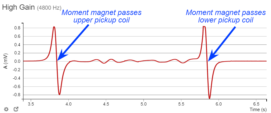
 between times when magnet passes the top and the bottom coil.
  to zoom in to the signal so that it looks like the one in Figure E.2.
 and select the time interval between moments when the voltage curve crosses 0. The time interval will be shown among statistics for selected interval (see Figure E.3).
  . It is most efficient to make 12-15 drops first and only after that zoom in on each drop and record appropriate time interval
  into Excel spreadsheet to calculate the mean and standard deviation for your data series. If the emf curve for certain drop is crooked (i.e. has unusual shape and you are not certain about the time when the magnet passes through pickup coil) discard such drop. Also discard obvious outliers - data points that differ drastically (~50% or so) from the rest. I do not expect any outliers but if you see them you might want to check your experimental setup.
  . But both
  and
and  are measured with uncertainties:
  ,
, 
 is your measured distance between the pickup coils (you do not need to measure it multiple times),
  is the uncertainty of your length measurement – i.e. the distance between the smallest ticks on the ruler (1mm). Note, that since your ruler is probably shorter than
  you have to apply it twice, and in that case
  .
. is the mean value for the time interval you measured,
  is its standard deviation for your data series.
  but how do we calculate the uncertainty for the speed? We combine relative uncertainties (see https://www.nde-ed.org/GeneralResources/Uncertainty/Combined.htm for the general rules on how to combine/propagate uncertainties in calculations). For two measured quantities
  and
and  their ratio
  is:
is: where
where  and
and 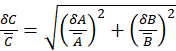


 ,
,  , and
, and  into provided Worksheet. Include the printout of this worksheet into your report. You do not need to include individual time interval measurements and the mean and standard deviation calculations into this worksheet and your report.
  between them.
  ,
,  , and
, and  in the Worksheet. You will measure and report terminal velocity in the same way in all experiments in this lab.
 for the blue magnet in this experiment using both Model 1 and Model 2 (use known characteristics for the tube and the magnet, calculate values for parameters
  ,
,  and scaling function
  ). Enter your theoretical estimates in the Worksheet. In your report compare experimental value for the terminal speed
  with theoretical estimates from Models 1 and 2. Do these models overestimate or underestimate
  ? Which model is more accurate?
  . Compared to the single blue magnet the mass of the combined magnet is doubled
  and the magnetic moment is
  . According to the point dipole approximation, the terminal velocity of the combined magnet should be less than ½ of that for a single blue magnet. Does your experimental result agree with this assessment? What is the value of the scaling function
  in Model 2? Compare accuracies of our models for the combined magnet in your report. Why is the difference between estimates by our models so large in this experiment?
  between them.
  the same as in Experiment 1. It is important for Experiment 3.3.
  . Does your data support this assertion?
  , and
, and  for the black magnet in coaxial tubes. Enter into the Worksheet. The distance
  traveled by the magnet in the experiments with ¾” tube, 1” tube, and in this experiment with both tubes together, is the same. Use data from your previous experiments to check the validity of our Model 3 assertion (M.24): the travel time for distance
  in the coaxial tubes equals to the sum of travel times for the same distance in the individual tubes.