Experiments in this lab involve dropping magnet in the straight copper tube positioned vertically. You will discover that due to interaction with the currents induced in the tube the magnet descends with constant (terminal) velocity. You will measure this velocity for several experimental setups and compare with the results obtained from theoretical calculations. In the following I present two theoretical models for evaluation of the terminal velocity of the magnet falling in the conducting tube.
Model 1 (Simple). Point dipole approximation.
(M.1) |
The current ![]() in this ring is
in this ring is
(M.2) |
where ![]() is the resistance of the ring (
is the resistance of the ring (![]() is the resistivity of copper,
is the resistivity of copper, ![]() is the circumference of the ring and
is the circumference of the ring and ![]() is its cross section area).
is its cross section area).
Current ![]() in the ring creates a magnetic field
in the ring creates a magnetic field ![]() at the location of our magnetic dipole. This magnetic field produces a force on the magnet
at the location of our magnetic dipole. This magnetic field produces a force on the magnet ![]() . We may calculate
. We may calculate ![]() and integrate over the whole tube (i.e. integrate over
and integrate over the whole tube (i.e. integrate over ![]() from
from ![]() to
to ![]() since we assume the tube is very long) to find the net retarding force
since we assume the tube is very long) to find the net retarding force ![]() from the currents in copper tube on the magnet.
from the currents in copper tube on the magnet.
From (M.2) it is clear that the magnitude of this retarding force is proportional to the velocity of the magnet: ![]() , where
, where ![]() is the coefficient that depends on the parameters of the tube and the magnet. Since the magnet descends with constant speed the net retarding force equals in magnitude to the weight of the magnet
is the coefficient that depends on the parameters of the tube and the magnet. Since the magnet descends with constant speed the net retarding force equals in magnitude to the weight of the magnet ![]() (
(![]() is the mass of the magnet):
is the mass of the magnet):
(M.3) |
While it is possible to use (M.3) to find ![]() we will, however, choose an alternative way of calculating terminal velocity - through energy conservation. As the magnet moves down the tube with constant speed its potential gravitation energy is transformed into heat in the tube (due to currents induced in the tube). The rate at which the heat is generated in one ring is:
we will, however, choose an alternative way of calculating terminal velocity - through energy conservation. As the magnet moves down the tube with constant speed its potential gravitation energy is transformed into heat in the tube (due to currents induced in the tube). The rate at which the heat is generated in one ring is:
|
(I have substituted ![]() for the ring resistance). The rate at which the heat is generated in the whole tube is the integral over all such rings
for the ring resistance). The rate at which the heat is generated in the whole tube is the integral over all such rings ![]() . This rate should be equal to the rate at which the force of gravity does work (i.e. the rate at which our magnet loses its potential gravitation energy). This rate is
. This rate should be equal to the rate at which the force of gravity does work (i.e. the rate at which our magnet loses its potential gravitation energy). This rate is ![]() . Therefore:
. Therefore:
![]()
![]()
|
Solving for ![]() yields:
yields:
|
(M.4) |
Model 2. Magnet of finite size.
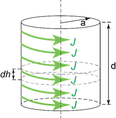
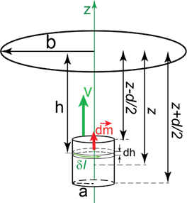
The magnetic dipole moment of our magnet can be thought of as one of the current loop ![]() (see Figure I.1). For the cylindrical magnet we assume the net current
(see Figure I.1). For the cylindrical magnet we assume the net current ![]() is distributed uniformly along the surface of the cylinder of length
is distributed uniformly along the surface of the cylinder of length ![]() (see Figure M.2). Current density (current per unit length of the cylinder) is
(see Figure M.2). Current density (current per unit length of the cylinder) is ![]() . We may present our cylindrical magnet as a stack of very thin current-carrying rings with the thickness
. We may present our cylindrical magnet as a stack of very thin current-carrying rings with the thickness ![]() . The current in such ring is
. The current in such ring is ![]() . Magnetic dipole moment of such ring is
. Magnetic dipole moment of such ring is
|
(M.5) |
This expression follows from the assumption that magnetic dipole moment is distributed uniformly over the length of the magnet.
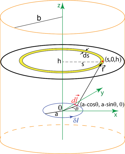
Now we will calculate magnetic field due to small segment of the current-carrying ring ![]() at some arbitrary observation point (denoted by the red dot in Figure M.3). Assume the current-carrying ring of radius a is located in the xy plane with its center at origin. The position of the
at some arbitrary observation point (denoted by the red dot in Figure M.3). Assume the current-carrying ring of radius a is located in the xy plane with its center at origin. The position of the ![]() segment is determined by the angle
segment is determined by the angle ![]() with the x-axis (see Figure M.3) so the segment’s coordinates are:
with the x-axis (see Figure M.3) so the segment’s coordinates are:
![]()
![]()
The position of the observation point is ![]() . We have oriented our coordinate axes so that y-coordinate of the observation point is 0 to simplify calculations. Vector
. We have oriented our coordinate axes so that y-coordinate of the observation point is 0 to simplify calculations. Vector ![]() from the ring segment
from the ring segment ![]() to the observation point is thus:
to the observation point is thus:
![]()
The distance between ![]() segment and the observation point is:
segment and the observation point is:
![]() =
=![]()
According to the Biot-Savart Law magnetic field at the observation point due to current ![]() in the segment
in the segment ![]() is
is
![]()
Therefore:
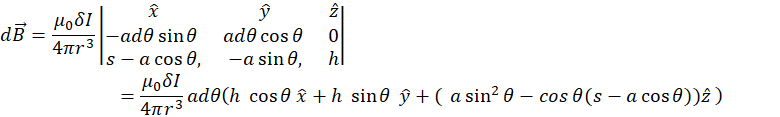
We are going to calculate the flux of this magnetic field through the circular cross-section of the tube (Figure M.3). For the flux calculations we only need z-component of the magnetic field:
![]()
To obtain z-component of the net magnetic field ![]() at the observation point due to the current carrying ring of radius a in the xy-plane we sum contribution due to all
at the observation point due to the current carrying ring of radius a in the xy-plane we sum contribution due to all ![]() , i.e. we integrate over angle
, i.e. we integrate over angle ![]() :
:
![]()
Since ![]() we can reduce integration to
we can reduce integration to ![]() interval:
interval:
![]()
Due to cylindrical symmetry for a given value of h the magnitude of ![]() depends only on the distance to the axis of symmetry s. Therefore, the flux
depends only on the distance to the axis of symmetry s. Therefore, the flux ![]() of the magnetic field due to current
of the magnetic field due to current ![]() in the magnet element (a ring of radius a ) through the coaxial tube element (a ring of radius b) at distance h is:
in the magnet element (a ring of radius a ) through the coaxial tube element (a ring of radius b) at distance h is:
![]()
Here ![]() is the area of the ring with radius s and thickness ds (highlighted in yellow in Figure M.3). Therefore:
is the area of the ring with radius s and thickness ds (highlighted in yellow in Figure M.3). Therefore:
![]()
From (M.5) the current in the ring is ![]() . Here
. Here ![]() is the net magnetic dipole of the magnet. Therefore:
is the net magnetic dipole of the magnet. Therefore:
|
(M.6) |
|
(M.7) |
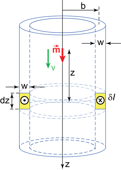
Here we assumed the distance between the center of the ring of radius b and the center of the magnet is z, therefore the magnet is represented as a stack of current carrying rings that extend from z-d/2 to z+d/2 along the axis of symmetry as shown in Figure M.4.
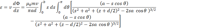
The magnet moves with constant speed v along the axis of symmetry of the system. The rest of the derivation follows in the footsteps of the Model 1. In analogy with (M.1) the emf induced in the ring:
![]()
From (M.7) we obtain
![]()
From (M.6) we have:
![]()
Therefore:
In analogy with Model 1, the rate at which the heat is generated in the element of the tube (a ring with radius b) is:
![]()
Where ![]() is the resistance of the ring (see Figure M.1). Therefore:
is the resistance of the ring (see Figure M.1). Therefore:
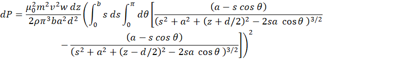
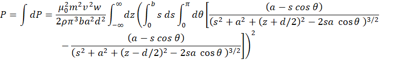
To find the rate of heat generation in the whole tube we add contributions of all tube elements (rings of radius b located at different distances z from the center of the magnet):
|
(M.8) |
Now we express all parameters with the dimension of length in terms of tube radius b:
(M.9) |
Substituting (M.9) into (M.8) yields:
 |
(M.10) |
We can rewrite (M.10) as
(M.11) |
where ![]() is dimensionless function of two dimensionless parameters
is dimensionless function of two dimensionless parameters ![]() and
and ![]() :
:
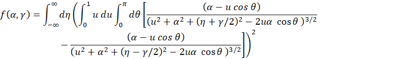 |
(M.12) |
As in Model 1 we now equate the rate at which the force of gravity does work with the rate of heat generation in the tube given by (M.11):
![]()
Solving for ![]() yields:
yields:
(M.13) |
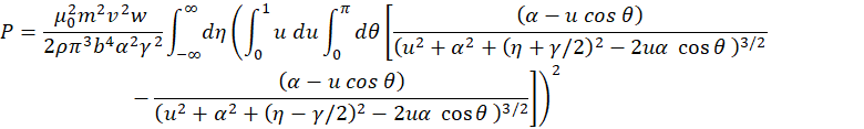
To facilitate easy comparison with the result (M.4) of the simple Model 1 we rewrite (M.13) as:
![]()
The first term in this product is the value for the terminal velocity obtained from our point dipole approximation Model 1 (see M.4). The second term is the dimensionless scaling function of two dimensionless parameters ![]() and
and ![]() . We will name this function
. We will name this function ![]() :
:
(M.14) |
Parameters ![]() and
and ![]() represent the ratios of magnet’s radius and height to the radius of the tube. For very small values of
represent the ratios of magnet’s radius and height to the radius of the tube. For very small values of ![]() and
and ![]() the point dipole approximation used in Model 1 is justified and scaling function
the point dipole approximation used in Model 1 is justified and scaling function ![]() should be close to 1 as both Models should yield very similar results. For large values of parameters
should be close to 1 as both Models should yield very similar results. For large values of parameters ![]() and/or
and/or ![]() (
(![]() ) we expect differences in terminal velocity values produced by two Models. Thus, our attempt to account for the finite size of the magnet in Model 2 lead to much more sophisticated but, hopefully, more accurate mathematical model.
) we expect differences in terminal velocity values produced by two Models. Thus, our attempt to account for the finite size of the magnet in Model 2 lead to much more sophisticated but, hopefully, more accurate mathematical model.
What are the assumptions (approximations) still used in Model 2? We assume the wall thickness of the tube is very small: ![]() . In the experiments performed in this lab this assumption seems to be justified since for copper tubes used in our experiments
. In the experiments performed in this lab this assumption seems to be justified since for copper tubes used in our experiments ![]() . We also assume that the magnet moves along the axis of symmetry of the tube without turning and shifting off the center. We will insert plastic tube inside the copper tube to ensure this assumption is satisfied.
. We also assume that the magnet moves along the axis of symmetry of the tube without turning and shifting off the center. We will insert plastic tube inside the copper tube to ensure this assumption is satisfied.
I evaluated scaling function ![]() numerically. You may find Python code used in evaluation of
numerically. You may find Python code used in evaluation of ![]() on canvas. The results are shown in Excel file Scaling.xlsx (also on canvas). Here is the graph of
on canvas. The results are shown in Excel file Scaling.xlsx (also on canvas). Here is the graph of ![]() :
:
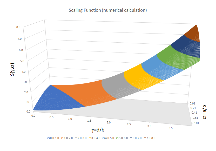
As expected, ![]() is 1 for
is 1 for ![]() Moreover, the shape of
Moreover, the shape of ![]() looks like hyperbolic paraboloid (shifted 1 unit up) which suggests that
looks like hyperbolic paraboloid (shifted 1 unit up) which suggests that ![]() could be well approximated by:
could be well approximated by:
|
(M.15) |
Fitting (M.15) to the accurate values of ![]() on the region
on the region ![]() , i.e. relevant region for magnets and tubes in our experiments yields
, i.e. relevant region for magnets and tubes in our experiments yields ![]() and
and ![]() (optimization calculations are also included in Scaling.xlsx). The resulting approximation is:
(optimization calculations are also included in Scaling.xlsx). The resulting approximation is:
|
(M.16) |
This approximation provides a good fit for the accurate calculated data of ![]() on indicated region with average relative residual (error) of 1%. At the same time (M.16) is easier to use than actual integration involved in evaluation of
on indicated region with average relative residual (error) of 1%. At the same time (M.16) is easier to use than actual integration involved in evaluation of ![]() Note that for values of
Note that for values of ![]() and
and ![]() beyond region
beyond region ![]() the deviation between (M.16) and accurate value of
the deviation between (M.16) and accurate value of ![]() may increase therefore one needs to either use accurate values of
may increase therefore one needs to either use accurate values of ![]() or approximate it with more fitting parameters.
or approximate it with more fitting parameters.
We may now summarize our result for Model 2 for the terminal velocity of the cylindrical magnet of radius ![]() and length
and length ![]() falling in the tube of radius
falling in the tube of radius ![]() :
:
|
(M.17) |
Model 3. Magnet falls inside two coaxial tubes.
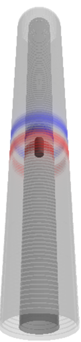
Magnet falling in two coaxial tubes.
Induced currents and their
polarities are shown in color.
Now we will build a simple model for evaluation of the terminal velocity of the magnet falling in the tube which is inside a larger coaxial tube (see Figure M. 6).
We know that the retarding force on the magnet moving in the conducting tube is proportional to the induced currents in the tube. Induced currents are proportional to the speed of the magnet. Therefore, the retarding force on the magnet is proportional to its speed. Thus, for the magnet falling in the tube at terminal velocity
(M. 18) |
where ![]() is some coefficient that depends on the parameters of the magnet and the tube (we may deduce
is some coefficient that depends on the parameters of the magnet and the tube (we may deduce ![]() from our results for Models 1 or 2, for example). Assume we have 2 tubes of different radii. At first, we drop the magnet in the tube 1. For this tube we have:
from our results for Models 1 or 2, for example). Assume we have 2 tubes of different radii. At first, we drop the magnet in the tube 1. For this tube we have:
(M. 19) |
Here ![]() is the coefficient for tube 1,
is the coefficient for tube 1, ![]() is the terminal velocity of the magnet falling in tube 1.
is the terminal velocity of the magnet falling in tube 1.
We now drop the same magnet into tube 2. For tube 2 we have similar equilibrium equation:
(M. 20) |
where ![]() is the coefficient for tube 2,
is the coefficient for tube 2, ![]() is the terminal velocity of the magnet in tube 2.
is the terminal velocity of the magnet in tube 2.
Now we insert the smaller tube inside the larger one. We make sure the tubes are coaxial. We drop our magnet into the smaller tube (see Figure M. 6). As the magnet falls the currents are induced in both tubes. Retarding forces due to induced currents in both tubes add, therefore the equilibrium equation is
(M. 21) |
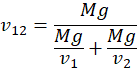
where ![]() is the terminal speed of the magnet as it falls in coaxial tubes. Solving for
is the terminal speed of the magnet as it falls in coaxial tubes. Solving for ![]() yields:
yields:
(M. 22) |
From (M. 19) and (M. 20): ![]() ,
, ![]() . Therefore:
. Therefore:
and
(M. 23) |
The time it takes our magnet to fall distance ![]() in two coaxial tubes
in two coaxial tubes
(M. 24) |
where ![]() ,
, ![]() are times it takes the magnet to drop the same distance
are times it takes the magnet to drop the same distance ![]() in tube 1 and tube 2 correspondingly.
in tube 1 and tube 2 correspondingly.
Tips.
In this lab you will measure induced emf. You will discover that emf is induced not only in circuits where you intend to measure it but also in connecting wires etc. To avoid getting confusing signals originating from induced emf in connecting wires lay them close together and/or wrap together to avoid unwanted induced emf. Avoid creating unintended loops that may induce emf from moving magnets.